A small and simple Python 3 code and illustrations are available
here to estimate the sensitivities. It will produce the figures below, except that you can change all of the input values, directly in the code.
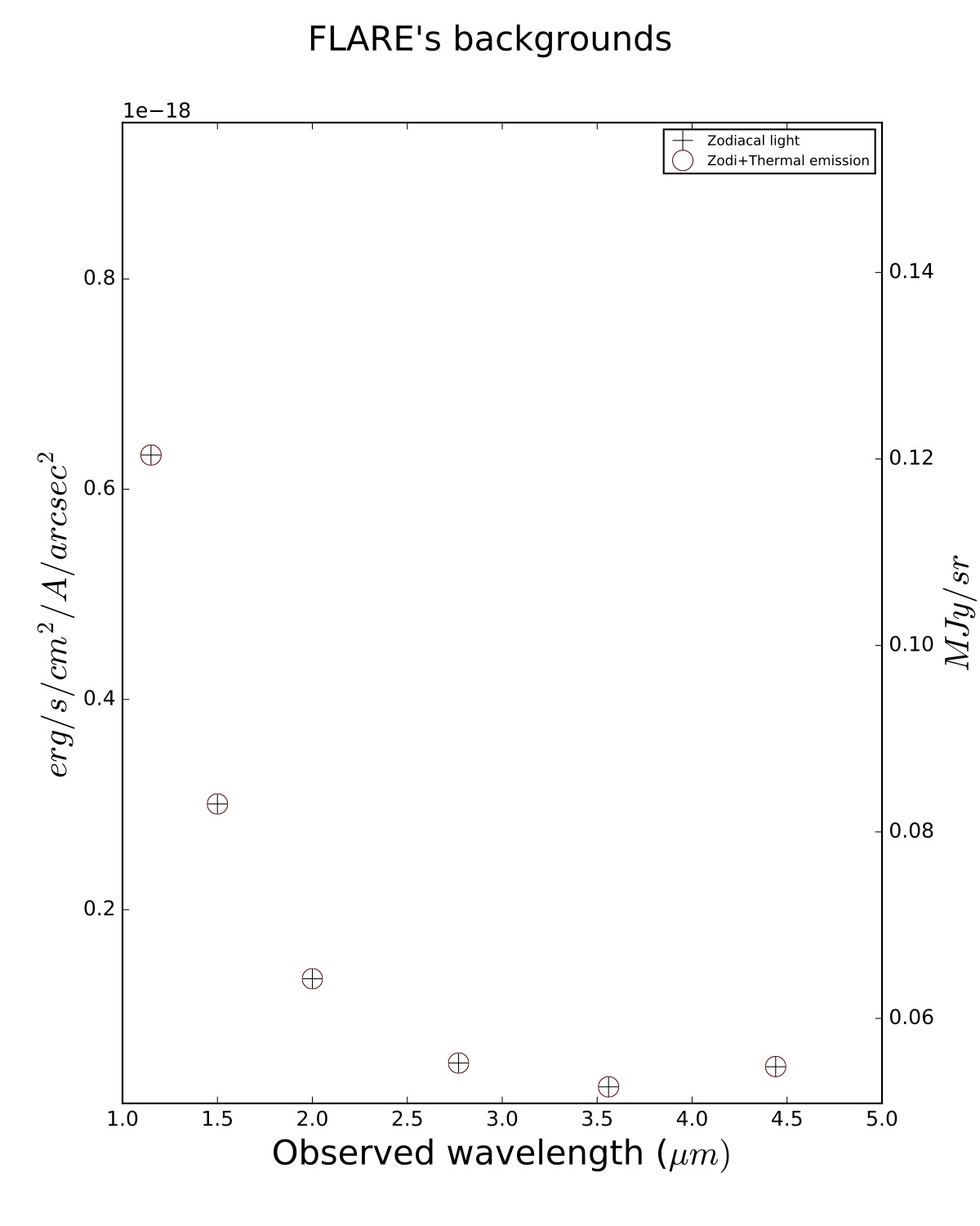
Fig1. - estimated background (zodiacal light + thermal emission from the telescope).
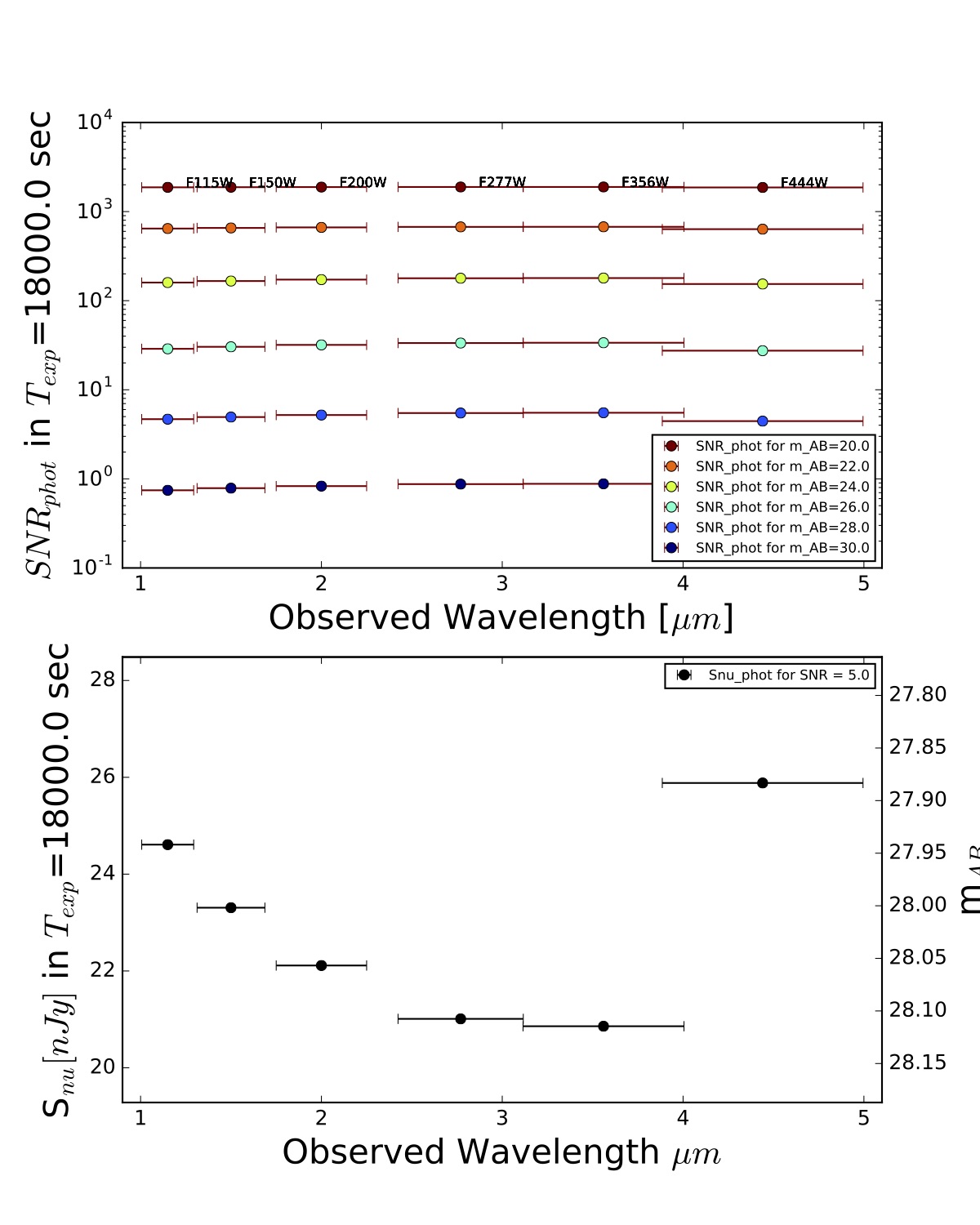
Fig2. - FLARE photometric sensitivity in 18 ksec (planned survey).
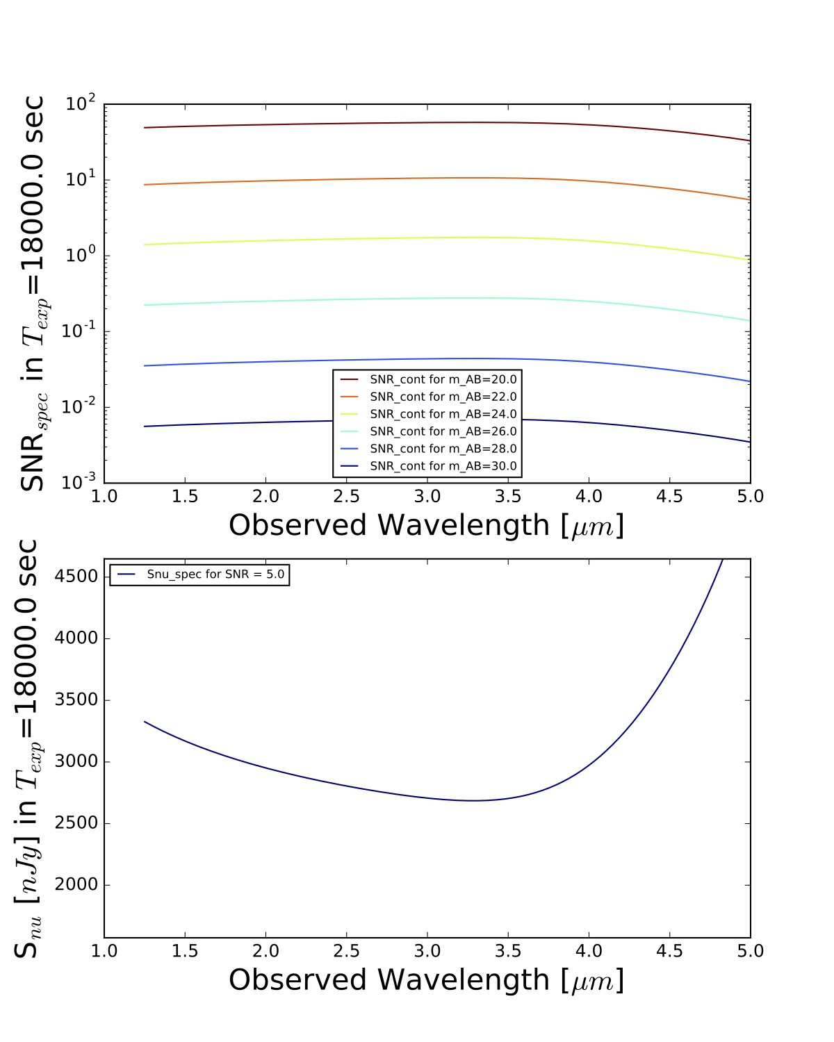
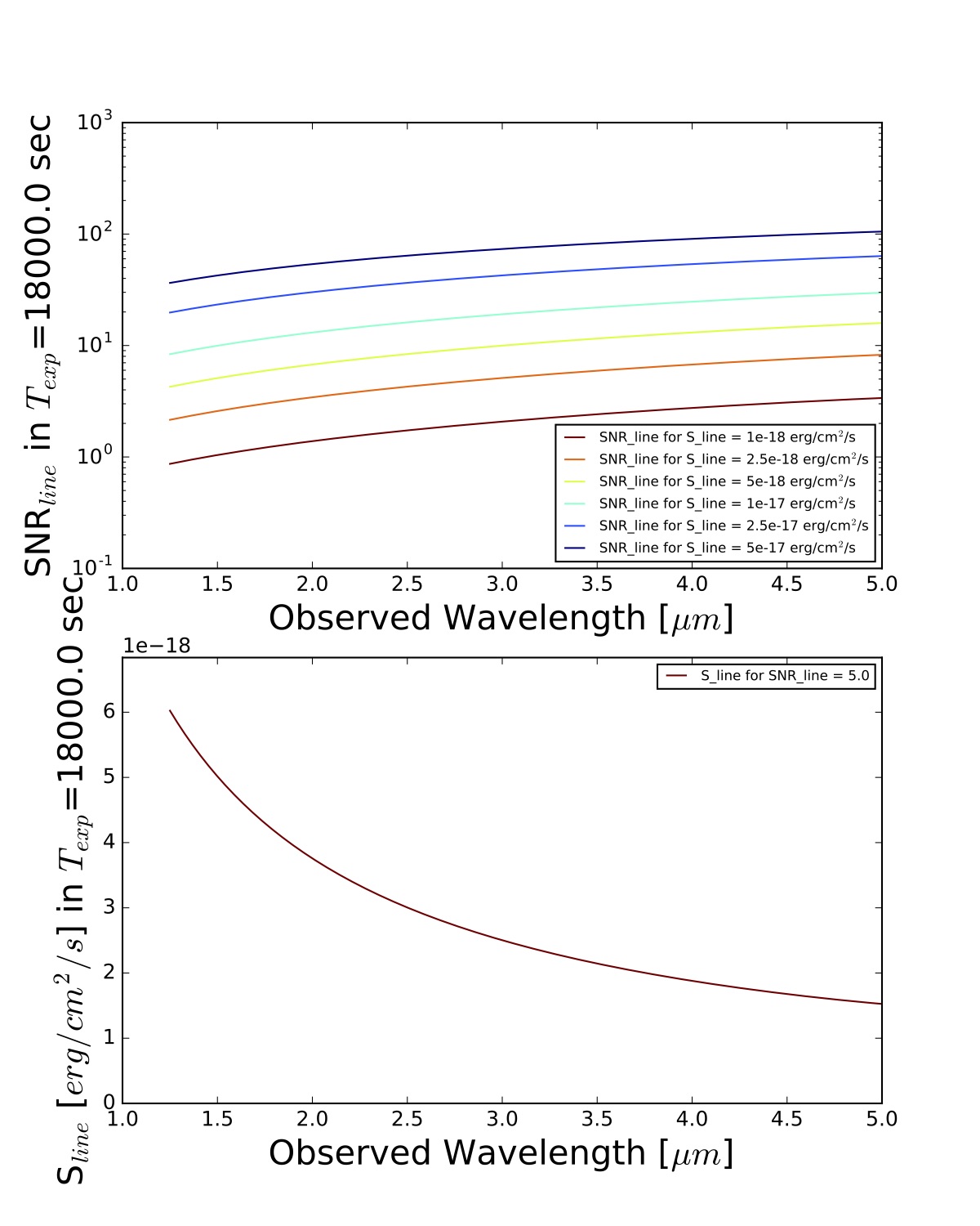
Fig4. - FLARE line sensitivity in 18 ksec (planned survey).
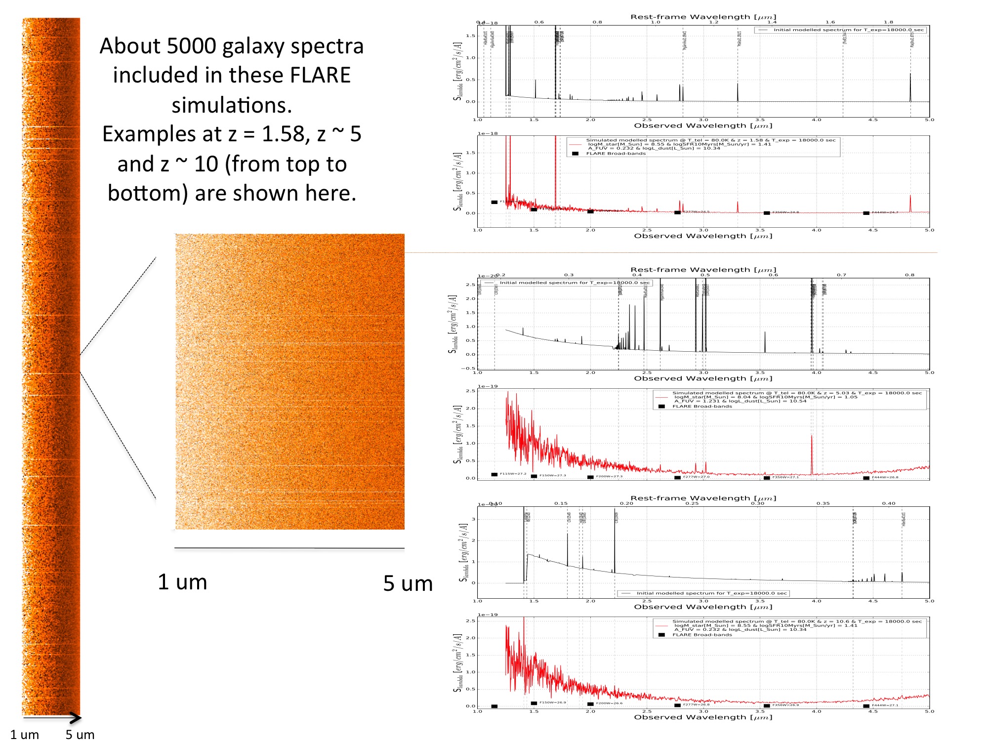
A more sophisticated code using CIGALE (http://cigale.lam.fr) is under development.
It will produce simulated observations based on a full emission model. The figure below is an example of the output.
Fig5. - How many galaxies will FLARE detect in Halpha and [OIII] in 1 sq. deg (the spectroscopic survey will be 1 to 2 sq. deg.)? Starting from observed luminosity functions,
we converted them in Halpha and O[III]luminosity functions assuming some boosting (factor x 3) to these large redshifts.
So, technically speaking, these numbers are still UV-selected galaxies and we might miss galaxies that will only be detected
from our spectroscopic blind survey. The symbols presents the respective sensitivities of FLARE in each of the redshift ranges for the two lines.
So, for instance, FLARE will detect > 10 000 galaxies at 7.5 < z < 8.5 and > 30 000 galaxies in Halpha at 5.5 < z < 6.5.
![Number of galaxies detected via Halpha and [OIII]](FigLF_allz.png)